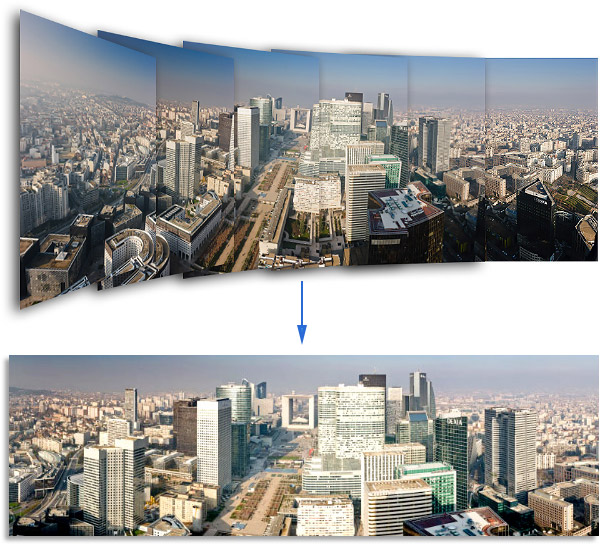
Computer Vision Basics (Part 1)- Image Formation
1.1 Primitives and Transformations
Geometric primitives are the basic building blocks used to describe 3D shapes. In this section, points, lines and planes will be introduced. We will also discuss some basic transformations.
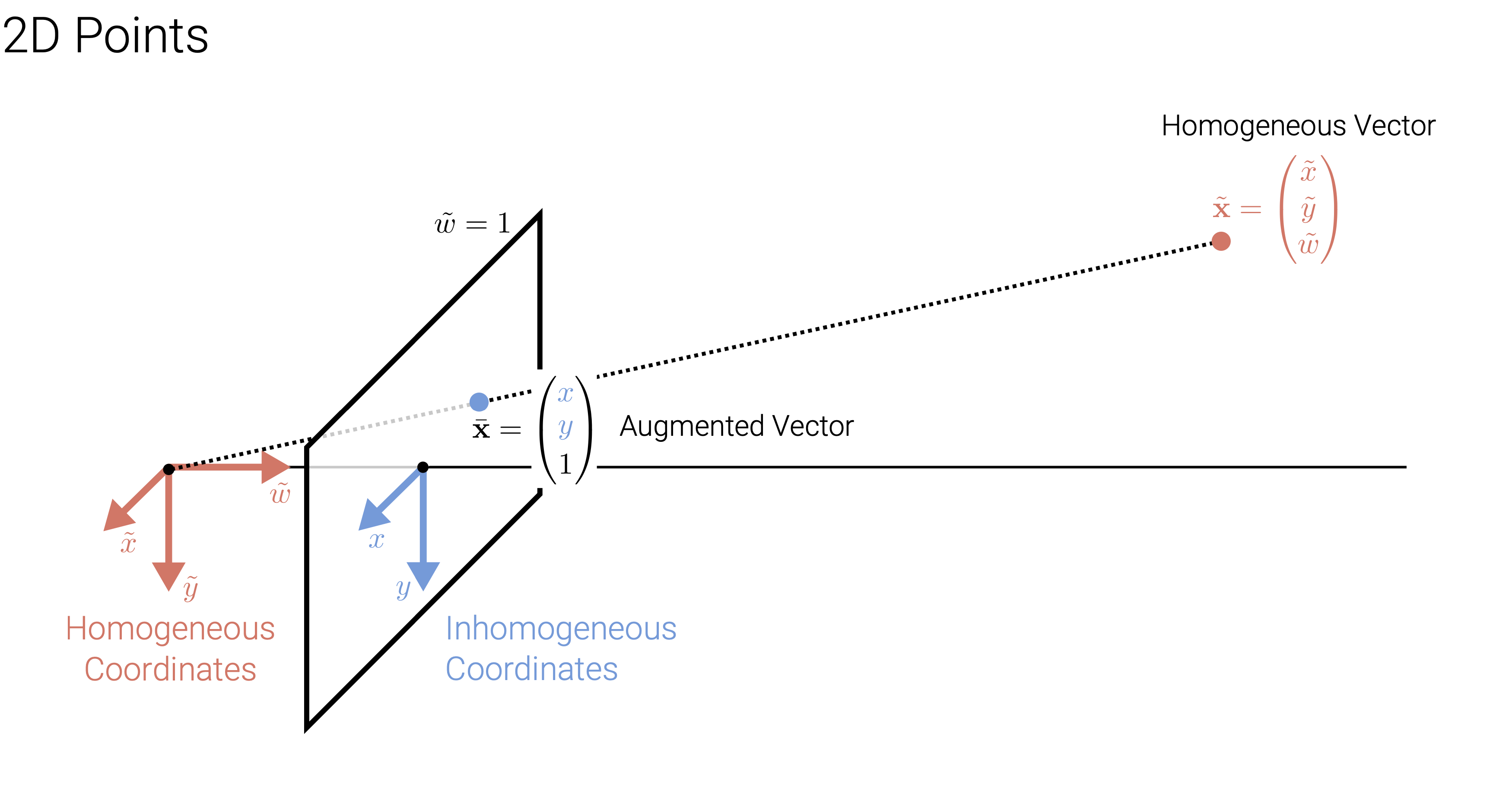
2D points can be written in inhomogeneous coordinated (as opposed to homogenous ones) by
\[x = \begin{pmatrix} x \\ y \end{pmatrix} \in \mathbb{R}^2\]or in homogenous coordinates as
\[x = \begin{pmatrix} \widetilde{x} \\ \widetilde{y} \\ \widetilde{w} \end{pmatrix} \in \mathbb{P}^2\]where \(\mathbb{P}^2 = \mathbb{R}^3 \backslash \{(0,0,0)\}\) is called projective space. Introducing a third coordinate here, we are in 3D space (except at 0,0,0). A tilde sign is a convention for a homogeneous coordinates. Homogeneous vectors are considered as equivalent when they differ onl up to scale. Thats why projective space is effectively only 2D.
An inhomogeneous vector x is converted to a homogeneous vector x as follows:
\[\widetilde{x} = \begin{pmatrix} \widetilde{x} \\ \widetilde{y} \\ \widetilde{w} \end{pmatrix} = \begin{pmatrix} x \\ y \\ 1 \end{pmatrix} = \begin{pmatrix} x \\ 1 \end{pmatrix} = \bar{x}\]with augmented vector \(\bar{x}\). We say augmented vector \(\bar{x}\) for all homogeneous vectors which last coordinate is equal to 1.
To convert in the opposite direction we divide by the last element \(\widetilde{w}:\)
\[x = \begin{pmatrix} x \\ 1 \end{pmatrix} = \begin{pmatrix} x \\ y \\ 1 \end{pmatrix} = \frac{1}{\widetilde{w}} \widetilde{x} = \frac{1}{\widetilde{w}} \begin{pmatrix} \widetilde{x} \\ \widetilde{y} \\ \widetilde{w} \end{pmatrix} = \begin{pmatrix} \widetilde{x}\mathbin{/}{\widetilde{w}} \\ \widetilde{y}\mathbin{/}{\widetilde{w}} \\ 1 \end{pmatrix}\]Like this, the last element of the homogeneous vector turens into a 1 and we can read off the x and y for the inhomogeneous coordinates. Homogeneous points whose last element is \(\widetilde{w} = 0\) are called ideal points or points at infinity. These poinits can’t be represented with inhomogeneous coordinates as we can’t divide by \(\widetilde{w}\).
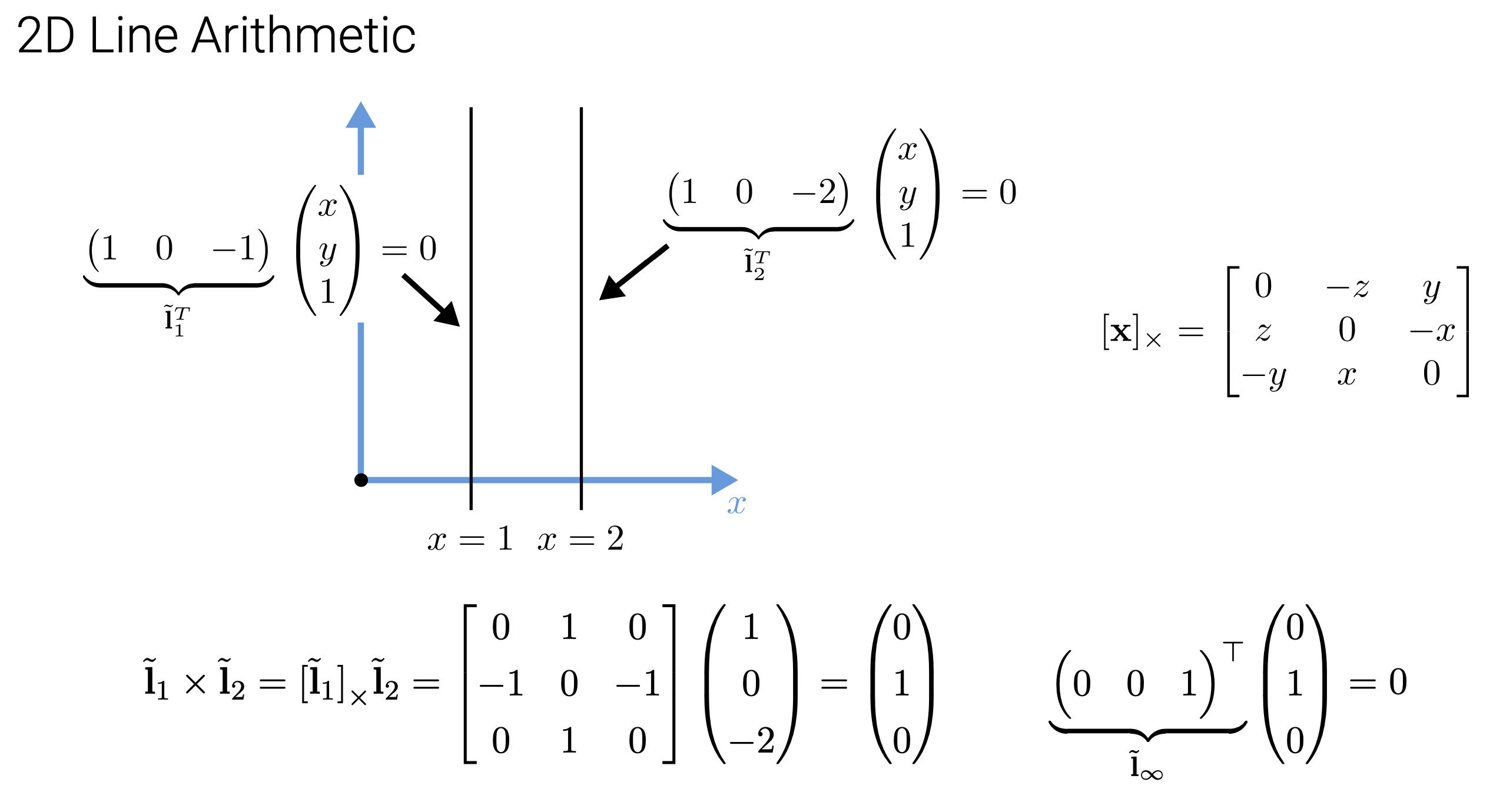
Now after the 2D points, we turn on to 2D lines. So, similar to the 2D points we can also represent 2D lines via the homogeneous coordinates as follows:
\[\{\bar{x} \hspace{0.2cm}\vert\hspace{0.2cm} \widetilde{\mathbf{l}}^\intercal \bar{x} = 0\} \Leftrightarrow \{x,y\hspace{0.2cm}\vert\hspace{0.2cm} ax+by+x=0\}\]where \(\widetilde{\mathbf{l}}=(a,b,c)^\intercal\).
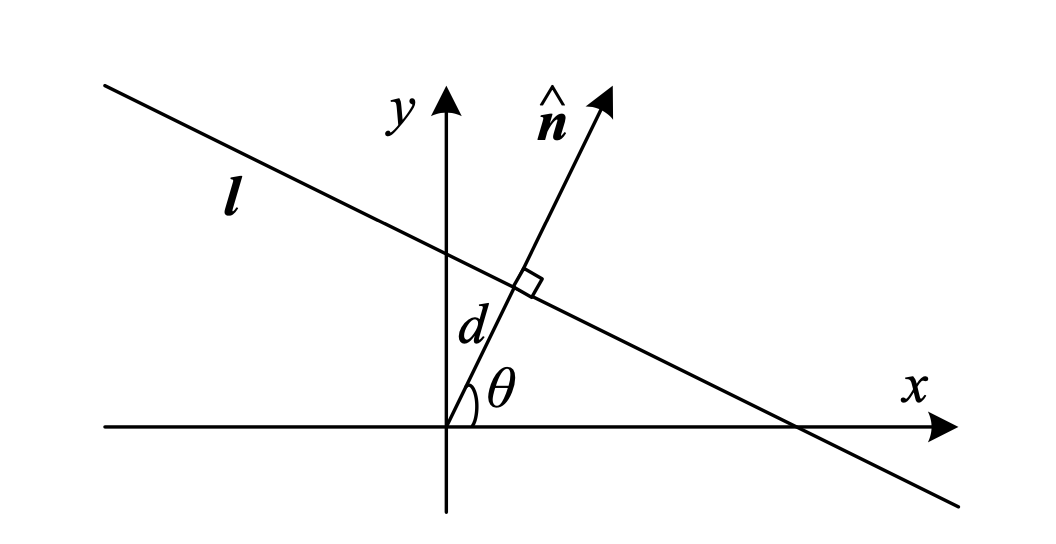
Here we can see that the inner product of the vector \(\widetilde{\mathbf{l}}\) with the augmented vector \(\bar{x}\) gives us the line equation. Note that we can use any vector (not only the augmented one). We can normalize the line equation vector so that \(\widetilde{\mathbf{l}} = (x_x,n_y,d)^\intercal = (\boldsymbol{n},d)^\intercal\) with \(\lVert n \rVert _2 =1\). In this case, \(\boldsymbol{n}\) is the normal vector perpendicular to the line and \(d\) is its distance to the origin. An exception is the line at infinity \(\widetilde{\mathbf{l}}_\infty = (0,0,1)^\intercal\) which passes through all the ideal points i.e we can’t normalize these lines since we have to divide by zero.
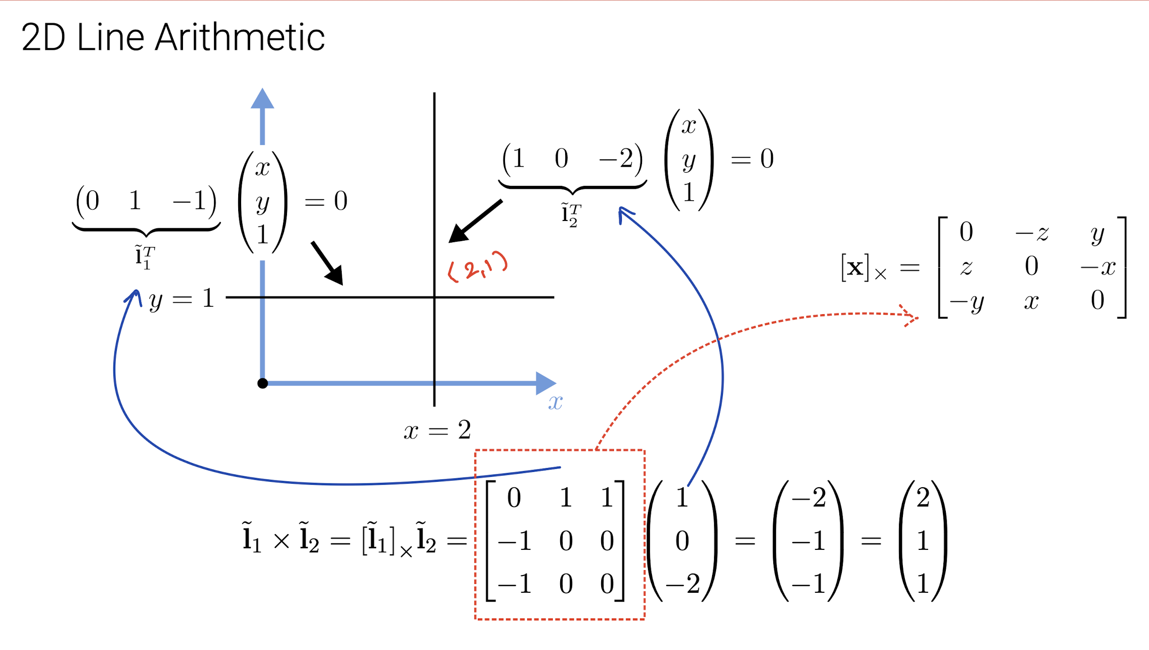
Another important concept is the cross product. When using homogeneous coordinates, we can compute the intersection of two lines as \(\widetilde{\mathbf{x}} = \widetilde{\mathbf{l}}_1 \times \widetilde{\mathbf{l}}_2\) where the cross product is expressed as the product of a skew-symmetric matrix and a vector.
Similarly, the line joining two points can be written as \(\widetilde{\mathbf{l}} = \bar{\mathbf{x}}_1 \times \bar{\mathbf{x}}_2\).
How can we prove that indeed line joining two 2D points can be expressed as there cross products?
Click to get the answer!
Consider two lines in 2D homogeneous coordinates, $$\widetilde{\mathbf{l}}_1 = [a_1, b_1, c_1]^T$$ and $$\widetilde{\mathbf{l}}_2 = [a_2, b_2, c_2]^T$$ The lines can be represented as: $$\begin{align*} \widetilde{\mathbf{l}}_1 &: a_1x + b_1y + c_1 = 0 \\ \widetilde{\mathbf{l}}_2 &: a_2x + b_2y + c_2 = 0 \end{align*}$$ Now, consider a point $$\widetilde{x} = [x, y, 1]^T$$ that lies on both lines. This means: $$\begin{align*} \widetilde{\mathbf{l}}_1^T \widetilde{x} &= 0 \\ \widetilde{\mathbf{l}}_2^T \widetilde{x} &= 0 \end{align*}$$ This implies that $ \color{blue} \widetilde{\mathbf{x}}$ is orthogonal to both $\color{blue} \widetilde{\mathbf{l}}_1$ and $\color{blue} \widetilde{\mathbf{l}}_2$. The cross product of two vectors gives a vector which is orthogonal to both of the original vectors. Therefore, we can write: $$ [ \widetilde{x} = \widetilde{\mathbf{l}}_1 \times \widetilde{\mathbf{l}}_2 ] $$ This is the point of intersection of the two lines. Hence, the cross product provides a very convenient method for calculating the intersection point of two lines, which is why it's used in this context. It also generalizes easily to 3D, where the cross product of two planes gives their line of intersection.
More complex algebraic objects can be represented using polynomial homogeneous equations. For example, a conic section can be represented as a homogeneous quadratic equation in 2D as:
\[\{\bar{\mathbf{x}}\vert\bar{\mathbf{x}}^\intercal \mathbb{Q} \bar{\mathbf{x}} = 0\}\]where $\mathbb{Q}$ is a symmetric matrix. The conic section can be a circle, ellipse, parabola or hyperbola depending on the eigenvalues of $\mathbb{Q}$. This is useful for multi-view geometry and camera calibration. For more details see Hartley and Zisserman
3D Points
3D points in inhomogeneous coordinates can be represented as
\[\mathbf{x} = \begin{pmatrix} x \\ y \\ z \end{pmatrix} \in \mathbb{R}^3\]or in homogeneous coordinates as
\[\widetilde{\mathbf{x}} = \begin{pmatrix} \widetilde{x} \\ \widetilde{y} \\ \widetilde{z} \\ \widetilde{w} \end{pmatrix} \in \mathbb{P}^3\]with projective space \(\mathbb{P}^3 = \mathbb{R}^4 \backslash \{(0,0,0,0)\}\)
3D Planes
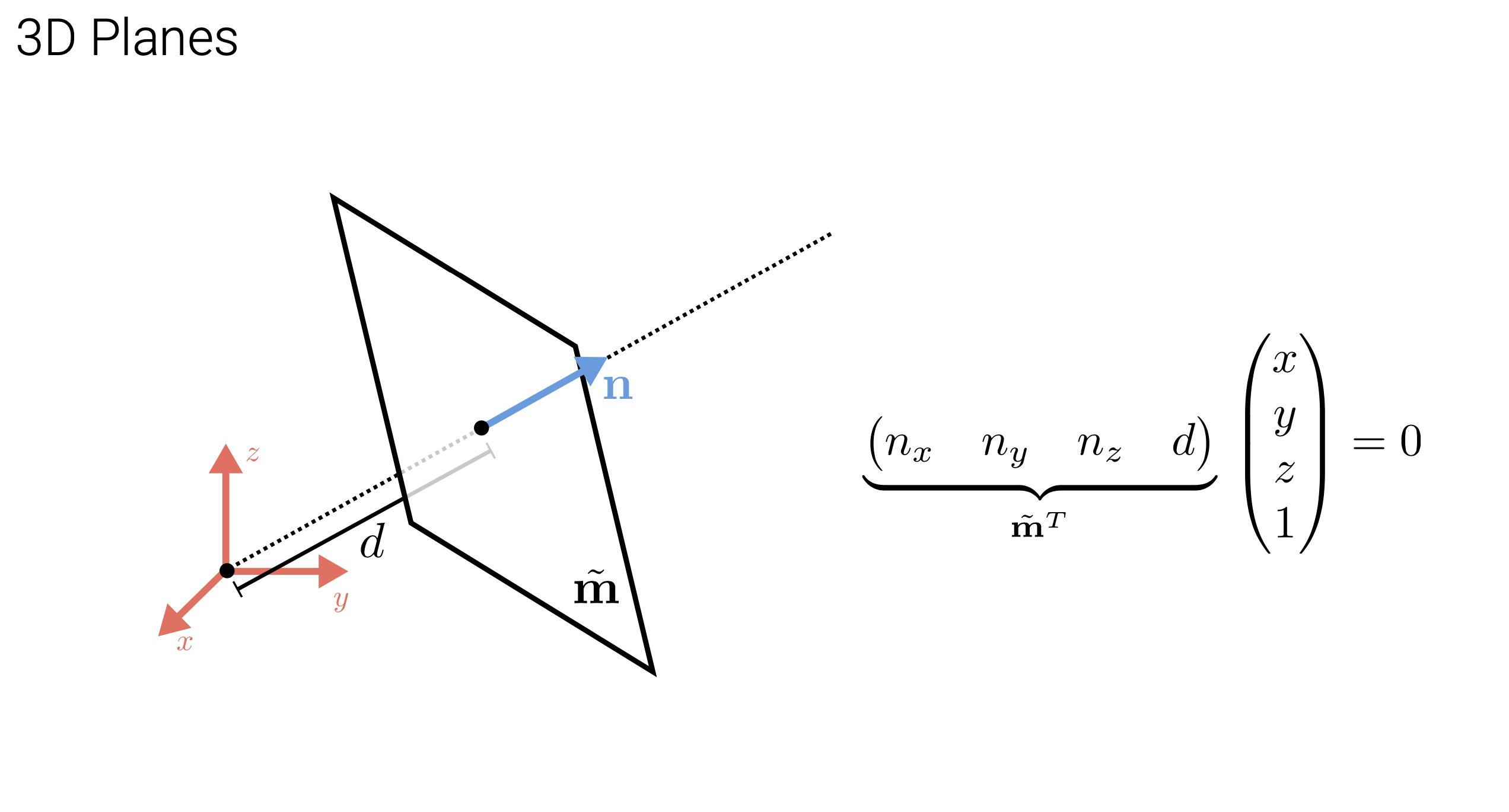
3D planes can also be represented in homogeneous coordinates as \(\widetilde{\mathbf{m}} = (a,b,c,d)^\intercal :\)
\[\{\mathbf{x}\hspace{0.2cm}\vert\hspace{0.2cm}\widetilde{\mathbf{m}}^\intercal\bar{\mathbf{x}}= 0\}\Leftrightarrow \{x,y,z\vert ax + by + cz + d = 0\}\]Again we can normalize \(\widetilde{\mathbf{m}}\) so that \(\widetilde{\mathbf{m}} = (n_x,n_y,n_z,d)^\intercal = (\boldsymbol{n},d)^\intercal\) with \(\|\boldsymbol{n}\|_2 = 1\). In this case, n is the normal perpendicular to the plane and d is the distance of the plane from the origin.
An exception is the plane at infinity, which is represented by \(\widetilde{\mathbf{m}} = (0,0,0,1)^\intercal\) which passes through all idead points for which \(\widetilde{w} = 0\).
3D Lines
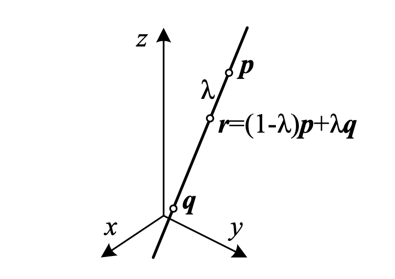
3D lines are less elegant than either 2D lines or 3D planes. One possible representation is to express points on a line as a linear combination of two points p and q on the line:
\[\{\mathbf{x}\vert\mathbf{x}=(1-\lambda)p + \lambda q \wedge \lambda \in \mathbb{R} \}\]However, this representation uses 6 parameters for 4 degrees of freedom.
A more compact representation is to use the two-plane parameterization or Plücker coordinates. More on this can be read in Hartley and Zisserman
The 3D analog of 2D conics is a quadrix surface. They are useful in the study of multi-view geometry. They also serve as useful modeling primitives in terms of compact representations. E.g Superquadrics, in order to represent geometric objects in terms of simple primitives.
2D Transformations
We will go through some common 2D transformations and their homogeneous representations.
Translation (2D Translation, 2 Degrees of Freedom)
Translation is a simple transformation that shifts the origin of the coordinate system by a fixed amount. In homogeneous coordinates, translation is represented by a matrix multiplication with a translation matrix:
\[x' = x + t \Leftrightarrow \bar{\mathbf{x}}' = \begin{bmatrix} \mathbf{I} & t \\ 0^\intercal & 1 \end{bmatrix} \bar{\mathbf{x}}\]With homogeneous coordinates we can easily chain and invert transformations.
Euclidean Transformation (2D Rotation + 2D Translation, 3 Degrees of Freedom)
Euclidean transformations are rigid body transformations that preserve distances and angles. They are represented by a matrix multiplication with a Euclidean transformation matrix:
\[x' = \mathbf{R}x + t \Leftrightarrow \bar{\mathbf{x}}' = \begin{bmatrix} \mathbf{R} & t \\ 0^\intercal & 1 \end{bmatrix} \bar{\mathbf{x}}\]where \(\mathbf{R}\) is a 2x2 rotation matrix and \(t\) is a 2D translation vector.
\(\mathbf{R} \in SO(2)\) is an orthonormal rotation matrix with \(\mathbf{R}^\intercal\mathbf{R} = \mathbf{I}\) and \(\det(\mathbf{R}) = 1\). Euclidean transformations preserve Euclidean distances and angles.
Similarity Transformation (2D Rotation + 2D Translation + 2D Scaling, 4 Degrees of Freedom)
Similarity transformations are Euclidean transformations that also preserve scale. They are represented by a matrix multiplication with a similarity transformation matrix:
\[x' = s\mathbf{R}x + t \Leftrightarrow \bar{\mathbf{x}}' = \begin{bmatrix} s\mathbf{R} & t \\ 0^\intercal & 1 \end{bmatrix} \bar{\mathbf{x}}\]where \(\mathbf{R}\) is a 2x2 rotation matrix, \(t\) is a 2D translation vector and \(s\) is a scaling factor. Even though they preserve angles, but now distances change as we have introduced a scaling factor. \(\mathbf{R} \in SO(0)\) is a rotation matrix and s is an arbitrary scaling factor.
Affine Transformation (2D Rotation + 2D Translation + 2D Scaling + 2D Shear, 6 Degrees of Freedom)
Affine transformations are similarity transformations that also preserve parallel lines. They are represented by a matrix multiplication with an affine transformation matrix:
\[x' = s\mathbf{R}x + t \Leftrightarrow \bar{\mathbf{x}}' = \begin{bmatrix} \mathbf{A} & t \\ 0^\intercal & 1 \end{bmatrix} \bar{\mathbf{x}}\]where \(\mathbf{A}\) is a 2x2 matrix and \(t\) is a 2D translation vector. Affine transformations preserve parallel lines, but not angles or distances.
Projective Transformation (Homography,2D Rotation + 2D Translation + 2D Scaling + 2D Shear + 2D Perspective, 8 Degrees of Freedom)
\[\widetilde{\mathbf{x}}' = \mathbf{H}\widetilde{\mathbf{x}} (\bar{\mathbf{x}} = \frac{1}{\widetilde{w}}\widetilde{\mathbf{x}})\]where \(\mathbf{H} \in \mathbb{R}^{3\times3}\) is an arbitrary homogeneous 3 × 3 matrix. Projective transformations preserve straight lines.
2D Transformations on Co-Vectors
Considering any perspective 2D transformation:
\[\widetilde{\mathbf{x}}' = \mathbf{H}\widetilde{\mathbf{x}}\]where \(\mathbf{H} \in \mathbb{R}^{3\times3}\) is an arbitrary homogeneous 3 × 3 matrix.
The transformed 2D line equation is given by:
\[\widetilde{\mathbf{l}}'^\intercal \mathbf{x}'= \widetilde{\mathbf{l}}'^\intercal \widetilde{\mathbf{H}}\widetilde{\mathbf{x}} = (\widetilde{\mathbf{H}}^\intercal\widetilde{\mathbf{l}}')^\intercal = \widetilde{\mathbf{l}}^\intercal \widetilde{\mathbf{x}}= 0\]Therefore we have:
\[\widetilde{\mathbf{l}}' = \widetilde{\mathbf{H}}^{-\intercal} \widetilde{\mathbf{l}}\]Thus the action of a projective transformation on a co-vector such as a 2D line or 3D normal can be represented by the transposed inverse of the matrix.
Overview of 2D Transformations
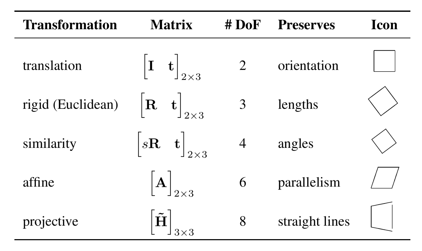
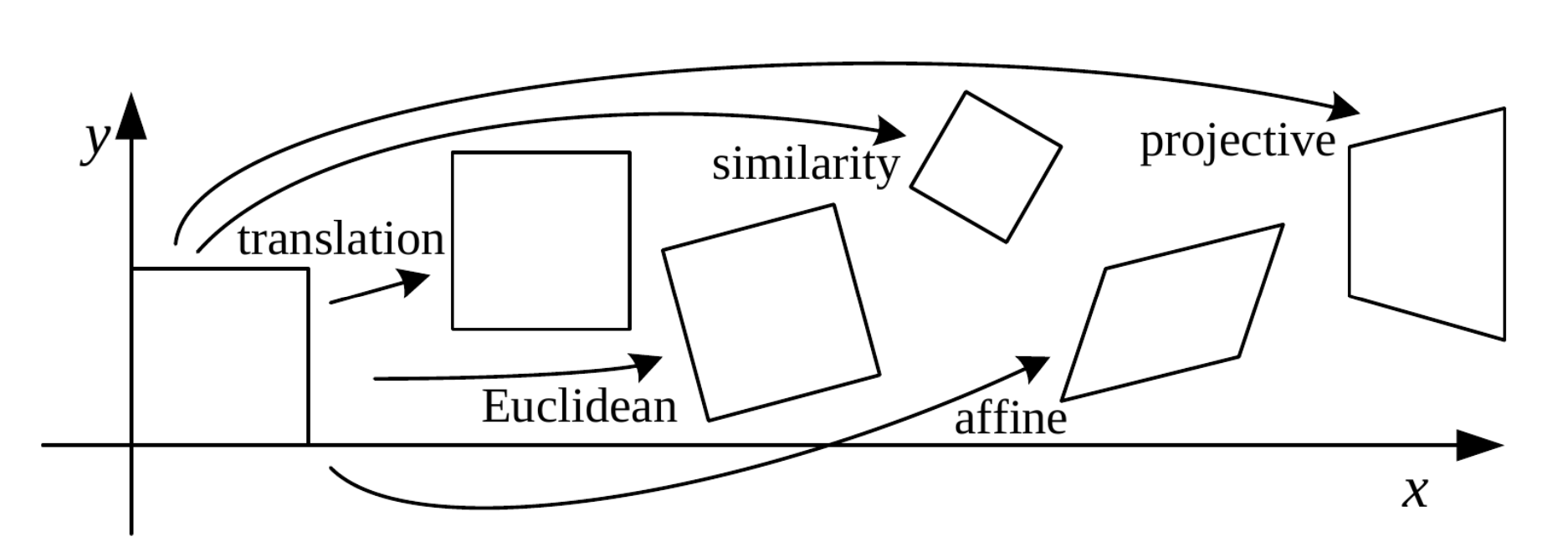
These 2D transformations form nested set of groups as shown in the figure above. The group of Euclidean transformations is a subgroup of the group of similarity transformations, which is a subgroup of the group of affine transformations, which is a subgroup of the group of projective transformations. And the transformations preserve the properties below them. For example, Euclidean transformations preserve Euclidean distances and angles, while similarity transformations preserve angles but not distances.
And as we go up from projective to translation transformation, more restrictions are imposed on the transformation.
Overview of 3D Transformations
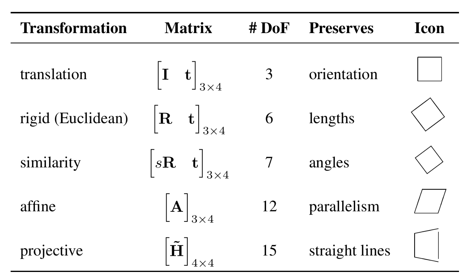
3D transformations are defined analogously to 2D transformations. 3 x 4 matrices are extended with a fourth \([0^\intercal 1]\) row for homogeneous transforms. Also the transformations preserve the properties below them. For example, Euclidean transformations preserve Euclidean distances and angles, while similarity transformations preserve angles but not distances.
Direct Linear Transform for Homography Estimation
How can we estimate a homography from a set of point 2D correspondences?
Let \(\mathbb{\chi} = \{\widetilde{\mathbf{x}}_i, \widetilde{\mathbf{x}}_i'\}_{i=1}^{N}\) denote a set of \(N\) point correspondences between two images, where \(\widetilde{\mathbf{x}}_i\) and \(\widetilde{\mathbf{x}}_i'\) are the homogeneous coordinates of the \(i\)-th point in the first and second image, respectively related by \(\widetilde{\mathbf{x}}' = \widetilde{H}\widetilde{\mathbf{x}}_i\).
As the correspondence vectors are homogeneous, they have the same direction but differ in magnitude. Thus, the equation above can be expressed as \(\widetilde{\mathbf{x}}'_i \times \widetilde{H}\widetilde{\mathbf{x}}_i = 0.\)
Using \(\widetilde{h}^\intercal_k\) to denote the k-th row of \(\widetilde{H}\), we can write linear equation in \(\widetilde{h}:\)
\[\underbrace{\left[\begin{array}{ccc} \mathbf{0}^{\top} & -\tilde{w}_i^{\prime} \tilde{\mathbf{x}}_i^{\top} & \tilde{y}_i^{\prime} \tilde{\mathbf{x}}_i^{\top} \\ \tilde{w}_i^{\prime} \tilde{\mathbf{x}}_i^{\top} & \mathbf{0}^{\top} & -\tilde{x}_i^{\prime} \tilde{\mathbf{x}}_i^{\top} \\ -\tilde{y}_i^{\prime} \tilde{\mathbf{x}}_i^{\top} & \tilde{x}_i^{\prime} \tilde{\mathbf{x}}_i^{\top} & \mathbf{0}^{\top} \end{array}\right]}_{\mathbf{A}_i} \underbrace{\left[\begin{array}{c} \tilde{\mathbf{h}}_1 \\ \tilde{\mathbf{h}}_2 \\ \tilde{\mathbf{h}}_3 \end{array}\right]}_{\tilde{\mathbf{h}}}=\mathbf{0}\]Each point correspondence yields two equations. Stacking all the equations into a 2N x 9 dimensional matrix A leads to the following constrained least squares problem:
\(\widetilde{h}^{*} = \underset{\widetilde{\mathbf{h}}}\arg \min \hspace{0.1cm}\|\mathbf{A}\widetilde{\mathbf{h}}\|_2^2 + \lambda(\|\widetilde{\mathbf{h}}\|_2^2 - 1)\) \(\widetilde{h}^{*} = \underset{\widetilde{\mathbf{h}}}\arg \min\hspace{0.1cm} \widetilde{\mathbf{h}}^\intercal\mathbf{A}^\intercal\mathbf{A}\widetilde{\mathbf{h}} + \lambda(\widetilde{\mathbf{h}}^\intercal \widetilde{\mathbf{h}} - 1)\)
Here we have fixed \(\|\widetilde{\mathbf{h}}\|_2^2 = 1\) as \(\widetilde{\mathbf{H}}\) i.e defined only up to scale. And the trivial soltuion to the above equation is \(\widetilde{\mathbf{h}} = \mathbf{0}\), which is not useful. Thus, we need to add a constraint to the problem to make it solvable. The solution to the above optimization problem is the singular vector corresponding to the smallest singular value of \(\mathbf{A}\). The resulting algorithm is called the Direct Linear Transformation (DLT) algorithm.
Panorama Stitching
